Diving Deep into Arrays

Arrays are among the most essential data structures in computing, typically introduced early on as straightforward collections of elements stored in contiguous memory. Yet beyond this simple definition lies a world of depth and nuance. In this article let's take a closer look at the inner workings of arrays, highlighting the concepts and hidden complexity that make them so fundamental.

The Essence of Arrays - Definition and Core Principles

At its core, an array is a fixed-size, homogeneous collection of elements stored in contiguous memory locations. Homogeneous means that every element in the array shares the same data type and size, ensuring consistent spacing between elements in memory. This property allows the computer to calculate the address of any element directly using simple arithmetic.

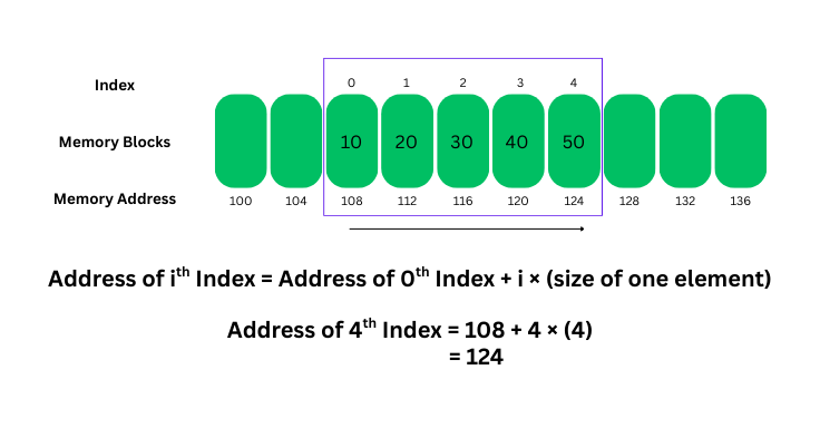
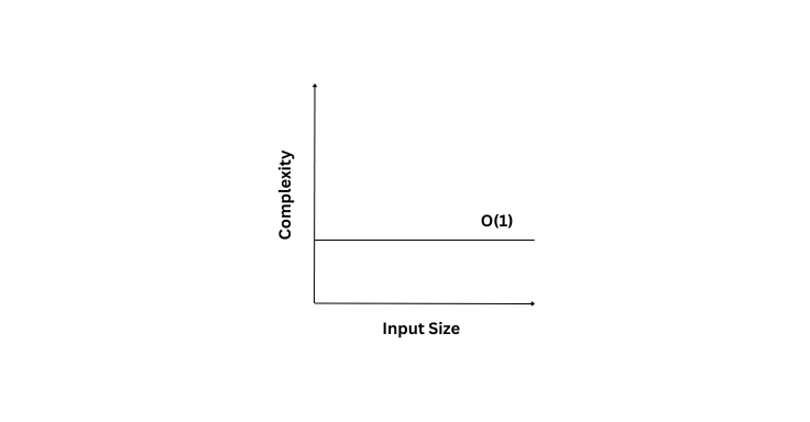
This direct addressing is what makes arrays so powerful. Accessing the i^th element requires no traversal or searching; it is simply a calculation, which results in O(1) constant-time access.

Viewing Array Memory in Practice (C Example)

In the below example, we declare an integer array of five elements. By compiling the program and running it in GDB, we can inspect the memory addresses of each array element and observe how the elements are stored contiguously. This hands-on approach reinforces the idea that array indexing is essentially pointer arithmetic and makes the memory layout of arrays tangible rather than abstract.

#include <stdio.h>

int main() {

    int arr[5] = {10, 20, 30, 40, 50};
    return 0;
}

To inspect variables and memory in GDB, let's compile the program using:

gcc -g -O0 array_example.c -o array_example

Next, Start GDB and set a breakpoint.

gdb ./array_example
break main
run

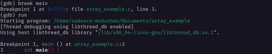
The program stops at the beginning of main, before any code executes. We can then use next to step over the array initialization.

After stepping over the line int arr[5] = {10, 20, 30, 40, 50};, the array is fully initialized in memory. We can now inspect the array addresses. To view the address of the entire array, we can use print &arr and to view the address of the first element, we can use print &arr[0].

Notice the first element and the array itself points to the same memory location, meaning it is 0 elements away from the location of the array itself.

We can examine raw memory directly using x/5d arr. This means “examine 5 integers in decimal starting from arr’s address.”

From the output, you can see how the array is laid out in memory:

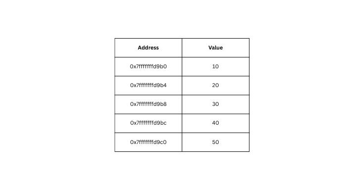
On a typical 64-bit system, each element of the array occupies 4 bytes, which is the standard size of an int. Because the elements are stored in contiguous memory locations, the address of each consecutive element increases by 4 bytes. This predictable spacing allows the program to calculate the address of any element directly using simple arithmetic, making array indexing highly efficient.

Static Arrays vs Dynamic Arrays

Beyond the foundational idea of arrays, they can be broadly categorized into static and dynamic types, depending on how memory is allocated and managed. In lower-level languages, this distinction is explicit and often left to the programmer, while in high-level languages it is usually managed automatically by the runtime or standard libraries. Still, the underlying principles remain the same, and understanding them is key to appreciating the trade-offs between efficiency, flexibility, and safety.

Static Arrays

Static arrays are those with a fixed size determined at the time of their creation. Once defined, their size cannot change at runtime, making them predictable but inflexible. This predictability allows the system to allocate exactly the required amount of memory up front, resulting in fast allocation and efficient access.

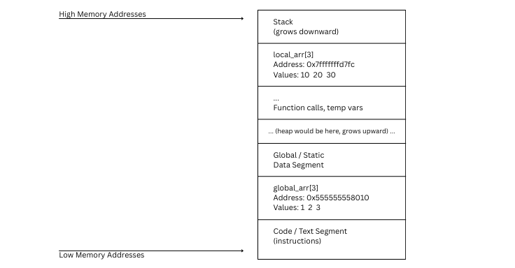
In lower-level languages like C, static arrays are often allocated on the stack (for local variables) or in the global data segment (for global variables). When a function exits, stack-allocated arrays are automatically released. However, the fixed nature of static arrays means you must know the maximum size in advance, oversizing can waste memory, while undersizing risks running out of space.

Consider the following C code:

#include <stdlib.h>

int global_arr[3] = {1, 2, 3};

void demo_function() {
    int local_arr[3] = {10, 20, 30};
}

int main() {
    demo_function();
    return 0;
}

In this example, we define two static arrays. A global array global_arr and a local array local_arr inside the function demo_function. The global array is allocated in the global data segment, which means its memory is reserved for the entire duration of the program. The local array, on the other hand, is allocated on the stack, so its memory is automatically reserved when the function is called and released when the function exits. Both arrays have a fixed size determined at compile time, and their elements are initialized at the point of declaration.

When we inspect these arrays in GDB, the differences become clear.

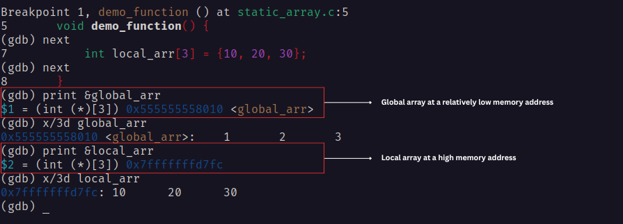
The global array resides at a relatively low memory address, reflecting its placement in the global data segment, and its memory is reserved for the entire duration of the program. In contrast, the local array appears at a high memory address, characteristic of stack allocation, which typically grows downward toward lower addresses as new functions are called. Using the x/3d command in GDB confirms that both arrays store their elements contiguously in memory: global_arr contains 1, 2, 3 and local_arr contains 10, 20, 30. This contiguous layout is what makes array indexing highly efficient, as the address of any element can be calculated directly from the base address. The difference in memory addresses also illustrates how stack-allocated arrays are temporary and released when the function exits, while global arrays persist throughout the program’s lifetime.

Dynamic Arrays

Dynamic arrays are arrays whose size can be determined and adjusted at runtime, offering flexibility that static arrays do not. Unlike static arrays, dynamic arrays are allocated on the heap, a larger memory pool managed by the system, which allows for much larger allocations than the stack. This makes dynamic arrays ideal when the number of elements cannot be known in advance.

Because dynamic arrays are managed at runtime, they typically require explicit memory management. The program must release the allocated memory when it is no longer needed to avoid leaks. They also incur some overhead, including the cost of allocation and potential fragmentation in memory. Despite this, dynamic arrays maintain the same fundamental property as static arrays, their elements are stored contiguously in memory, allowing efficient indexing and predictable traversal. When resizing is needed, a new block of memory is allocated and the existing data is copied over, enabling the array to grow or shrink as necessary.

Consider the following C example:

#include <stdlib.h>

void demo_dynamic() {
    int *dyn_arr = (int *)malloc(3 * sizeof(int));
    dyn_arr[0] = 100;
    dyn_arr[1] = 200;
    dyn_arr[2] = 300;

    free(dyn_arr);
}

int main() {
    demo_dynamic();
    return 0;
}

In this example, dyn_arr is a pointer to a dynamically allocated array. Its memory is allocated on the heap at runtime and remains valid until explicitly released with free(). Unlike stack-allocated arrays, heap memory persists beyond the scope of the function call, offering greater flexibility but requiring careful management.

When we observe this in GDB,

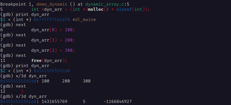
We first step to the line where the dynamic array is allocated using malloc. At this point, the pointer dyn_arr shows a valid heap address (0x7ffff7fe5af0), indicating that memory has been successfully reserved on the heap. As we step through the lines where elements are assigned (dyn_arr[0] = 100, dyn_arr[1] = 200, dyn_arr[2] = 300), the values are stored contiguously in memory. Using the x/3d dyn_arr command confirms this, showing the elements 100, 200, 300 sequentially at the heap address.

After calling free(dyn_arr), the memory is released back to the system, but the pointer still holds the old address. Accessing the memory through this pointer now results in undefined behavior, which is why using x/3d dyn_arr in GDB returned garbage values.

Arrays, whether static or dynamic, form the backbone of countless algorithms and applications due to their simplicity and efficiency. By understanding their inner workings: contiguous memory allocation, direct addressing, and the trade-offs between fixed and flexible sizing, developers can harness their power while navigating their limitations. From the predictable speed of static arrays to the adaptable nature of dynamic ones, arrays exemplify how fundamental design choices in data structures impact performance and scalability. Mastering these concepts not only deepens your appreciation for arrays but also equips you to make informed decisions in crafting efficient, robust code.